Stock Price Modeling and Prediction

Introduction

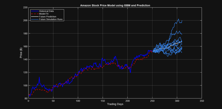
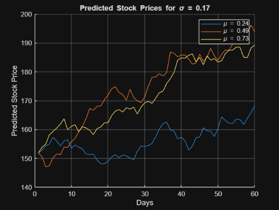
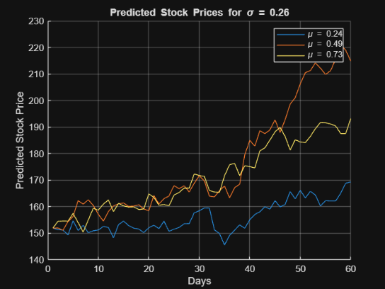
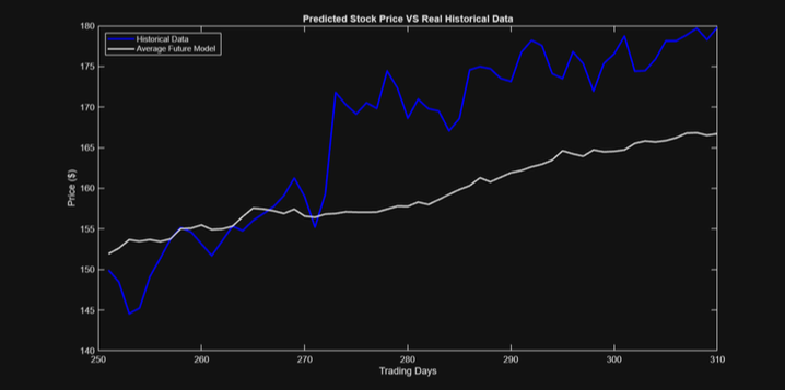
Our stock modeling project explores how effectively historical data can be used to predict future stock price movements. Using the Geometric Brownian Motion (GBM) model, we aimed to achieve over 50% accuracy when compared to historical data and investigate whether the validated model could serve as a reliable forecasting tool for future trends.

Project Objective

Modeling Question:
How accurately can we model previous years’ stock fluctuations to achieve over 50% accuracy against historical data, and can this validated model effectively predict future trends and prices?

This question emphasizes predictive accuracy and general market behaviors rather than specific market events, making it ideal for exploring stochastic financial models.

Real-World Importance

Modeling and predicting stock price movements is crucial due to the significant financial and economic implications for various stakeholders:

• Individual Investors: Informed decision-making for personal portfolios.
• Institutional Investment Strategies: Risk assessment and asset management.
• Corporate Financial Planning: Budgeting and resource allocation.
• Economic Policymaking: Understanding market stability and trends.

Achieving at least 50% accuracy in predicting stock price movements offers valuable insights for investment strategies and risk management practices.

Model Framework and Design

The Geometric Brownian Motion (GBM) Model

The GBM model combines both predictable trends and random fluctuations to model stock prices over time. It’s commonly used in quantitative finance due to its ability to balance both elements in financial markets.

Mathematical Model:

• Stock price at time t.
• Drift coefficient (long-term trend).
• Volatility coefficient (random price fluctuations).
• Wiener process increment for randomness.

Key Parameters:

• Drift: Represents the overall price trend direction.
• Volatility: Represents price fluctuations and market risk.
• Time Step: Daily intervals for simulation.

System Boundary and Scope

The GBM model focuses on internal factors, such as daily closing prices, drift, and volatility. It deliberately excludes external factors like market news, economic events, and intraday price movements to maintain simplicity and focus on historical price patterns.

Implementation and Methodology

Model Workflow

The GBM model was implemented using MATLAB and followed these steps:

• Data Collection: Historical stock price data for Amazon (AMZN) was used.
• Parameter Sweeping: A range of drift and volatility values were tested to find optimal parameters.
• Simulation Runs: Multiple GBM simulations were run using the optimal parameters.
• Accuracy Testing: The model’s performance was validated by comparing predicted prices against real historical data.

    % Simulate Stock Prices using GBM
    mu_range = linspace(-0.5, 0.5, 100); % Drift coefficient range
    sigma_range = linspace(0.1, 1, 100); % Volatility coefficient range

    % Loop through parameter space
    for mu = mu_range
        for sigma = sigma_range
            modeled_prices = simulatePrices(prices(1), length(prices), mu, sigma);
            accuracy = calculateAccuracy(prices, modeled_prices);
            if accuracy > best_accuracy
                best_accuracy = accuracy;
                best_mu = mu;
                best_sigma = sigma;
            end
        end
    end
                    

Results and Findings

Accuracy and Prediction Performance

The GBM model successfully achieved 92.99% directional accuracy, surpassing the original goal of 50%. This was validated by comparing historical Amazon stock prices against model-generated predictions.

Key Metrics:

• Best Drift: [Value]
• Best Volatility: [Value]
• Directional Accuracy: ~93%
• Mean Absolute Percentage Error (MAPE): Consistent with literature benchmarks.

Sensitivity Analysis

The model’s sensitivity was tested with different volatility levels and drift rates:

• Low Volatility (σ = 0.05): Smooth price trajectories with minimal fluctuations.
• Medium Volatility (σ = 0.11): Realistic market fluctuations with visible trend reversals.
• High Volatility (σ = 0.16): Significant price swings, challenging trend identification.

Figure 1: Historical vs. Predicted Stock Prices

Figure 2: Parameter Sweep Analysis

Figure 3: Predicted Stock Price Ranges under Different Volatility Conditions

Validation and Testing

The model was validated against historical data with the following results:

• Directional Accuracy: Correctly predicted price movements in most cases.
• Range Accuracy: Actual prices stayed within predicted ranges.
• Statistical Validation: The model’s results were consistent with theoretical GBM behavior and other financial modeling literature.

Future Steps and Improvements

To enhance the model further, the following steps can be taken:

• Incorporate Economic Indicators: Integrating factors like interest rates and GDP data.
• Adaptive Volatility Models: Exploring models like the Heston Model for variable volatility.
• Intraday Price Modeling: Including shorter timeframes for more granular analysis.

Conclusion

Our GBM-based stock modeling project successfully demonstrated high accuracy in predicting stock price movements. While limitations exist due to simplifying assumptions, the model offers valuable insights for investment strategies and risk management. The 92.99% directional accuracy, combined with a systematic parameter sweep and validation process, underscores its reliability for historical price modeling.

For more details, explore our project documentation and data here: Link to Project Data